The offshore DC structure is in the north of DC gas field, and DC target is located above the diapir in the north of DC diapir. The main target layer is the upper stratum of Neogene Miocene series. The target is the low-lying submarine fan developed during sedimentary period and controlled by flexure slope break, which is a structural plus lithologic trap. The wellhead water depth is 70m, and design vertical depth is -3600m, as shown in Figure 1.

 
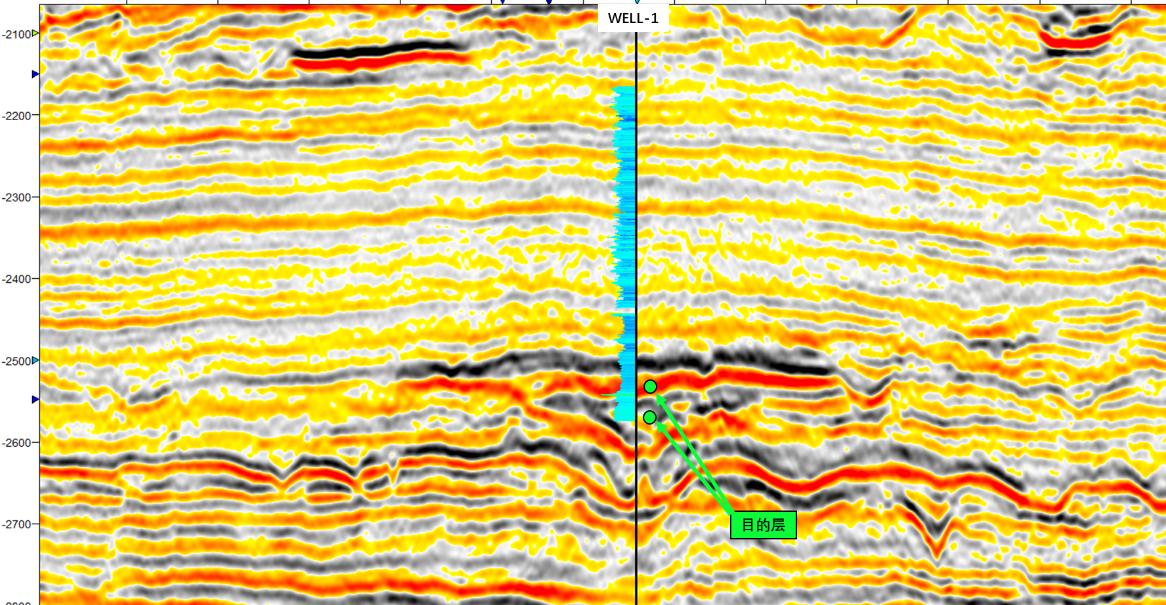
Figure 1 3D time domain seismic profile cross WELL-1

The formation temperature prediction of WELL-1 is based on the measured formation temperature of adjacent drilled DST and MDT, fitting the regression relationship between temperature and depth (Fig. 2), and predicting that the temperature from the target layer of WELL-1 to the bottom of the well is 156 ℃~164 ℃.

 
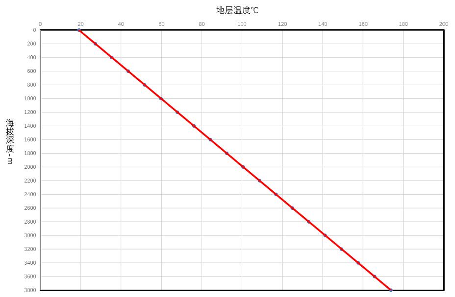
Figure 2 Prediction of Formation Temperature of Well-1

WELL-1 is located in overpressure area of the basin. The vertical pressure system has characteristics of abrupt distribution, that is, it changes rapidly from normal pressure system to abnormally high-pressure, ultra-high-pressure system, and the thickness of transition section is small or not obvious, as shown in Figure 3. Therefore, accurately predicting the change of formation pore pressure is crucial to ensure the safety of drilling engineering.

 
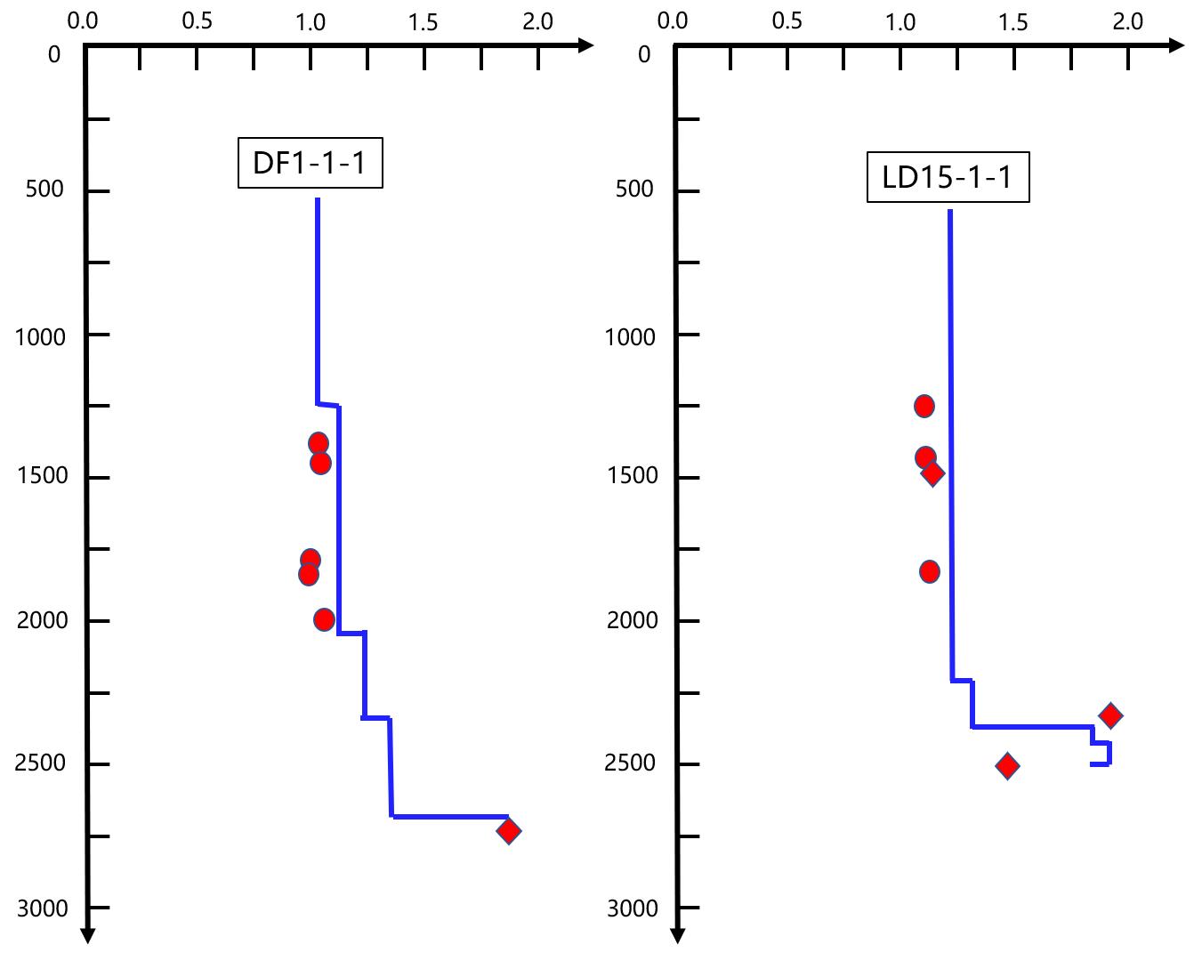
Figure 3 Distribution characteristics of abrupt vertical pressure

1、Velocity modelling and pre-stack depth migration

Starting from time migration CMP gathers, through a series of optimization processing such as residual NMO correction, random noise attenuation, residual multiple removal, etc., the initial velocity model of working area is established by integrating seismic stack velocity, sonic logging of adjacent wells, time horizon interpretation and other data using geostatistical methods. Based on this, the grid tomographic velocity inversion under horizon constraint is carried out, the best migration parameters are determined through experiments, the final PSDM migration depth volume is generated, and the prediction results of pre-drilling target depth are submitted. Figure 4 is the processing flow of pre-stack depth migration, Figure 5 is the profile of depth migration across WELL-1, and Table 1 is the prediction result of main target depth based from pre-stack depth migration.

 
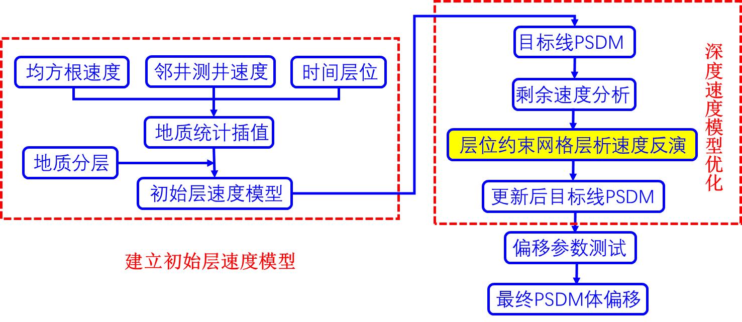
Figure 4 Pre-stack depth migration workflow

 
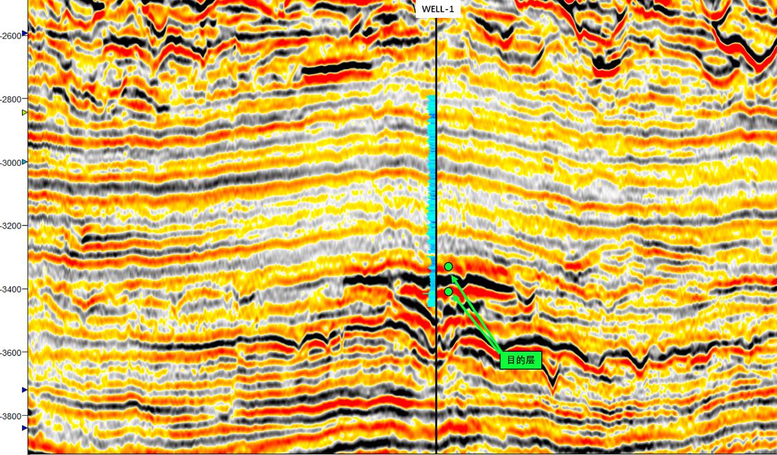
Figure. 5 Pre-stack depth migration profile through design well

 
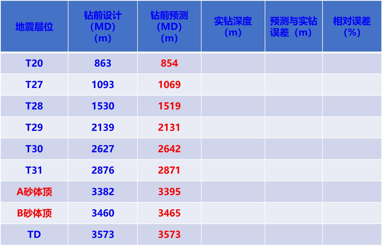
Table 1  Prediction table of pre-drilling target depth

2、Pre-stack deterministic inversion and pre-drill pressure prediction

3D pressure field prediction needs to calculate three pressure curves of reference wells by referring to analysis results of petrophysical and mechanical characteristics of wells. With the help of 3D seismic velocity, density, geothermal temperature, shale content and other parameters, under the control of stratigraphic structure and sedimentary sequence framework model, stress field modeling and geostatistics theory are applied to build 3D pore pressure, fracture pressure and overburden pressure models, and then extract the three pressure curves at the design well position from those three models.

Based on three adjacent wells of WELL-1, the optimized 3D CRP gathers are used to conduct pre-stack deterministic inversion through well seismic calibration, angle wavelet extraction, and low-frequency model construction, to obtain P-wave impedance, P-wave velocity, density, and Vp/Vs ratio volumes, and prepare for 3D pressure field prediction. Figure 6 shows P- wave velocity profile across wells.

 
Figure.  6 P-wave velocity profile across WELL-1

According to vertical distribution of pressure system in work area, Dutta pressure model that best matches with pressure test results is selected after variety of pressure model tests. This method considers petrophysical parameters, which can better describe the process of rapid transition in vertical direction, from normal pressure system to overpressure system. Figure 7 shows calculation results of three-pressure models of adjacent wells.

 
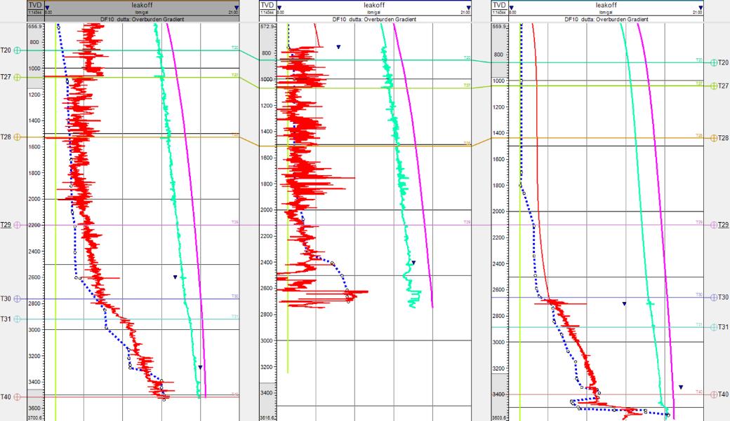
Figure. 7 Calculation results of pressure model of adjacent wells

Based on single well pressure model, combined with P-wave velocity, density, volume of shale and geothermal temperature, eastimate 3D pore pressure gradient, fracture pressure gradient and overburden pressure gradient, and finally extract three pressure curves at design well location to obtain pressure prediction results. Figure 8 shows pore pressure gradient profile through design well, Figure 9 shows the calculated 3D fracture pressure gradient, and Figure 10 shows the prediction results of three pre-drill pressures of design well.

 
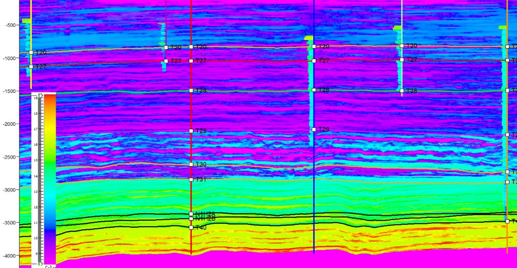
Figure 8 Predicted Pore Pressure Gradient Profile

 
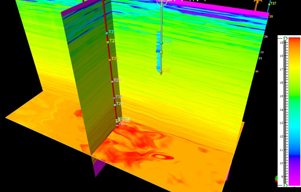
Figure 9 Results of 3D fracture pressure gradient

 
Figure 10 Prediction results of pressure in design well

3、Risk warning of weak interval

Use compressed sensing frequency extension algorithm to expand the bandwidth of seismic data and gain energy of high-frequency components. Impedance inversion is carried out after optimized data to obtain high-resolution P-wave impedance data, enhance recognition ability of thin interbed, and give early warning to weak layers that may be encountered during drilling to avoid engineering accidents.

According to analysis of leakage characteristics of adjacent WELL4, it is found that the response characteristics of P-impedance of the leakage section are, that the sub-high impedance in high impedance background, is the possible leakage layer (Fig. 11). The main reason for the leakage is: ①There are faults in leakage section；There is a large difference between sand and mud in leakage section；In P-impedance leakage window (P-impedance window of leakage section 9500~11000 m/s * g/cm³).

 
Figure 11 Analysis of impedance characteristics in lost circulation section of adjacent wells

Applying the conclusion to design well location, it is found that P-impedance of two intervals has similar characteristics with adjacent wells, namely depth of MD3335-3361m and MD3421-3500m. There is no obvious fault in first risk section, but it is inside impedance leakage window (9500-11000m/s * g/cc), and there is a relatively clear sand-shale interface. This conclusion was confirmed in later actual drilling process. When the bit depth is MD3328m, and mud weight is 1.81g/cm³, leakage occurred. At the depth of MD3441m, the drilling was completed ahead of plan due to leakage. Figure 12 shows broadband seismic and corresponding P-impedance profile of the first risk section.

 
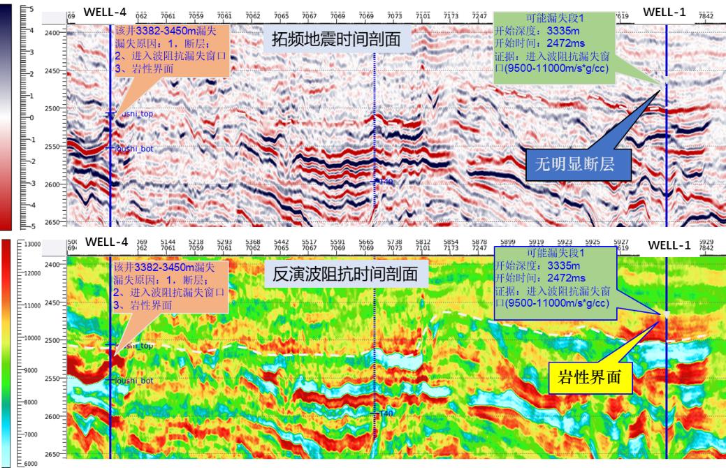
Figure 12 The first risk section of designed WELL-1

4、Depth and pressure model updating while drilling

The velocity information while drilling comes from two aspects: one is the logging curve while drilling; The second is the error between predicted and actual depth. On the basis of the structural framework, seismic velocity is constrained by new logging data that is closer to real formation velocity, and tomographic velocity inversion is further carried out, and the seismic data is updated by depth migration, according to magnitude of prediction error.

Collect daily drilling reports and various engineering information, timely adjust and update the pressure prediction results according to changes in mud weight, drilling time curve, LWD, mud logs, and DXC monitoring data, and issue updated prediction report to ensure the safety of drilling.

In process of well tracking for more than 40 days, it has experienced three depth migration imaging update, five pressure model reconstruction, and issued 16 prediction update reports. The task of well tracking has been successfully completed, and the depth and pressure prediction have exceeded the accuracy requirement of contract. Figure 13 shows the error comparison between pressure prediction and measured pressure, and the prediction error of pressure coefficient is between 0.01-0.06; Figure 14 demonstrates the comparison results of predicted and actual drilling depth, and depth prediction error is between 2-10m.

 
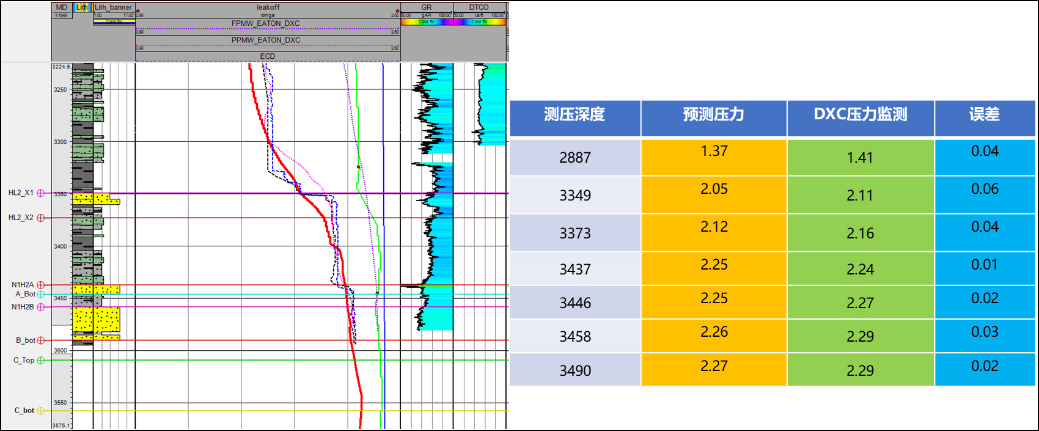
Figure 13 Pressure prediction results and error analysis

 
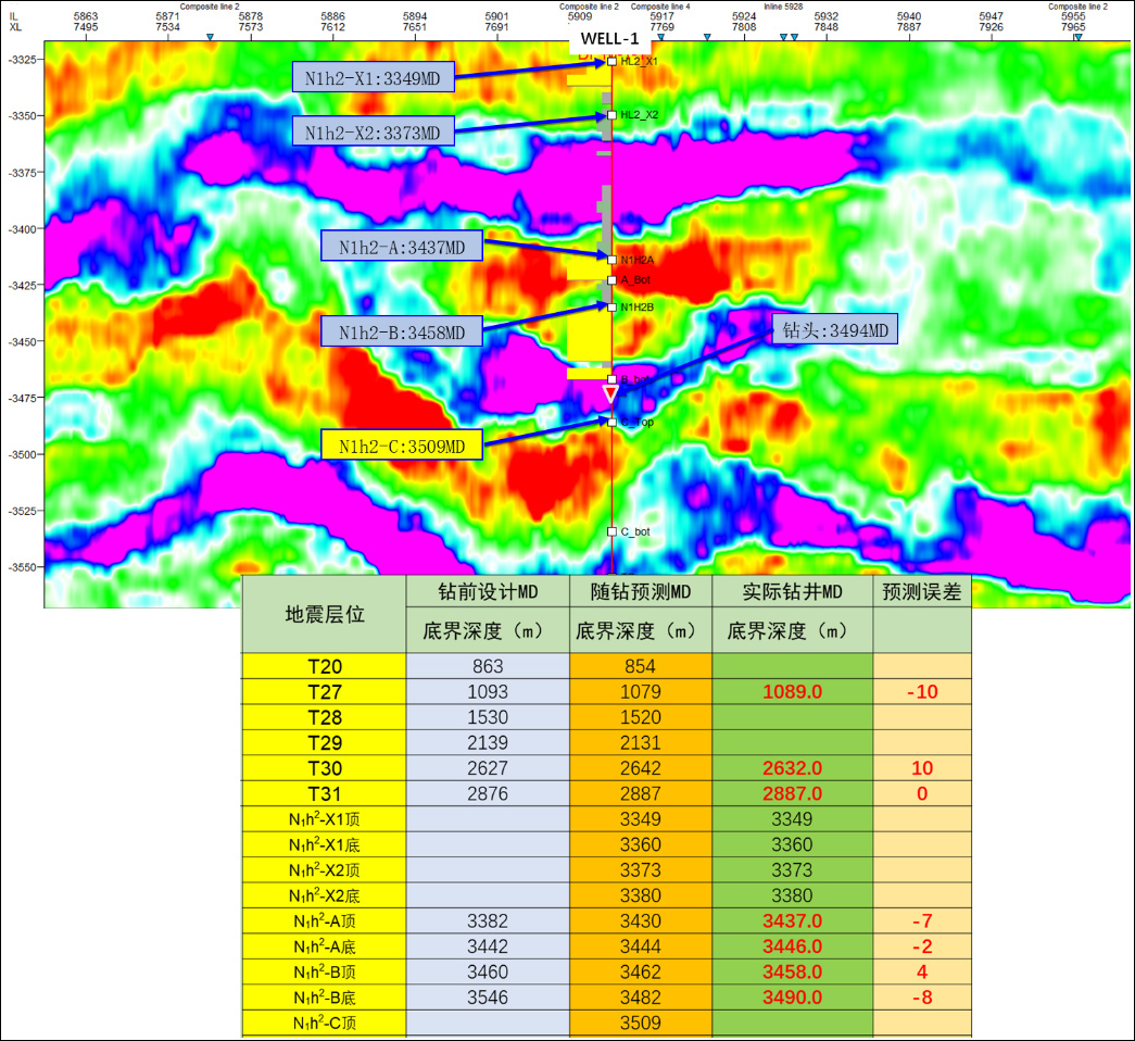
Figure 14 Analysis of depth prediction error